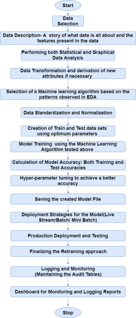
Linear Regression in Machine Learning

Linear Regression in Machine Learning is one of the most fundamental algorithms. It is the door to the magical world ahead, but before going further with the algorithm. Let’s have a look at the life cycle of the Machine Learning model.

This diagram explains the Machine Learning model from scratch and then taking the same model further with Hyperparameter tuning to improve the accuracy, and then deciding the deployment strategies for that model.

Once deployed, setting up the logging and monitoring frameworks to generate reports and dashboards based on projects requirement. 👇👇

Linear Regression 🤔🤓

Linear Regression is one of the most fundamental and widely known Machine Learning Algorithm.

Building blocks of Linear Regression are:

• Discreet/continuous independent variables.
• A best-fit regression line.
• Continuous dependent variable. i.e., A Linear Regression model predicts the dependent variable using a regression line based on the independent variables. The equation of the Linear Regression is:
  • Y = a + b*x + e 👌✌️
  • Where, a is the intercept, b is the slope of the line, and e is the error term. The equation above is used to predict the value of the target variable based on the given predictor variable(s).

Problem Statement 🤔🤓

This data is about the amount spent on advertising through different channels like TV, Radio and Newspaper. The goal is to predict how the expense on each channel affects the sales and is there a way to optimize that sale?

# necessary Imports
import pandas as pd
import matplotlib.pyplot as plt
import pickle
% matpllotlib inline

data= pd.read_csv('Advertising.csv') # Reading the data file

data.head() # checking the first five rows from the dataset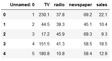

What are the features? 😜😝

• TV: Advertising dollars spent on TV for a single product in a given market (in thousands of dollars)
• Radio: Advertising dollars spent on Radio
• Newspaper: Advertising dollars spent on Newspaper

What is the response? 😷😷

• Sales: sales of a single product in a given market (in thousands of widgets)

data.info() # printing the summary of the dataframe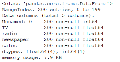

Now, let’s showcase the relationship between the feature and target column

# visualize the relationship between the features and the response using scatterplots
fig, axs = plt.subplots(1, 3, sharey=True)
data.plot(kind='scatter', x='TV', y='sales', ax=axs[0], figsize=(16, 8))
data.plot(kind='scatter', x='radio', y='sales', ax=axs[1])
data.plot(kind='scatter', x='newspaper', y='sales', ax=axs[2])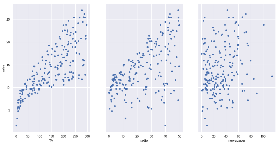

Simple Linear Regression 🤔🤗

Simple Linear regression is a method for predicting a quantitative response using a single feature (“input variable”). The mathematical equation is: 👇👇

𝑦 =𝛽0 + 𝛽1𝑥 👌👌

What do terms represent?

• 𝑦 is the response or the target variable
• 𝑥 is the feature
• 𝛽1 is the coefficient of x
• 𝛽0 is the intercept

𝛽0 and 𝛽1 are the model coefficients. To create a model, we must “learn” the values of these coefficients. And once we have the value of these coefficients, we can use the model to predict the Sales!

Multiple Linear Regression 🤗🤔

Till now, we have created the model based on only one feature. Now, we’ll include multiple features and create a model to see the relationship between those features and the label column. This is called Multiple Linear Regression.

𝑦=𝛽0+𝛽1𝑥1+…+𝛽𝑛𝑥𝑛 😵😲

Each 𝑥

represents a different feature, and each feature has its own coefficient. In this case:

𝑦=𝛽0+𝛽1×𝑇𝑉+𝛽2×𝑅𝑎𝑑𝑖𝑜+𝛽3×𝑁𝑒𝑤𝑠𝑝𝑎𝑝𝑒𝑟 😝👌

Let’s use Stats models to estimate these coefficients

# create X and y
feature_cols = ['TV', 'radio', 'newspaper']
X = data[feature_cols]
y = data.sales

lm = LinearRegression()
lm.fit(X, y)

# print intercept and coefficients
print(lm.intercept_)
print(lm.coef_)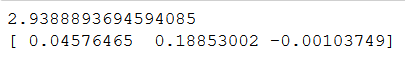

How do we interpret these coefficients? If we look at the coefficients, the coefficient for the newspaper spends is negative. It means that the money spent for newspaper advertisements is not contributing in a positive way to the sales.

A lot of the information we have been reviewing piece-by-piece is available in the model summary output: 👇👇

lm = smf.ols(formula='sales ~ TV + radio + newspaper', data=data).fit()
lm.conf_int()
lm.summary()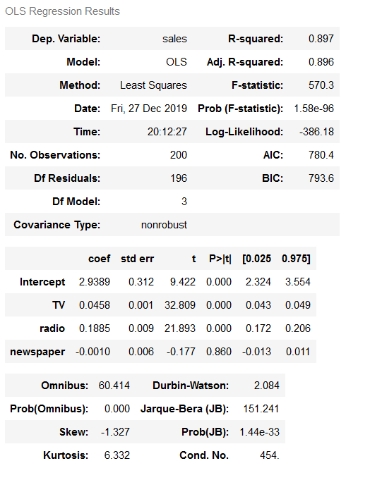

What are the things to be learnt from this summary? 😗😍

• TV and Radio have positive p-values, whereas Newspaper has a negative one. Hence, we can reject the null hypothesis for TV and Radio that there is no relation between those features and Sales, but we fail to reject the null hypothesis for Newspaper that there is no relationship between newspaper spends and sales.
• The expenses on bot TV and Radio ads are positively associated with Sales, whereas the expense on the newspaper ad is slightly negatively associated with the Sales.
• This model has a higher value of R-squared (0.897) than the previous model, which means that this model explains more variance and provides a better fit to the data than a model that only includes the TV.

Recommended Reading: How to start learning Python Programming 👈

Good Luck with your decision making let me know in the comment which project you choose in the end.

Follow Me ❤😊

If you like my post please follow me to read my latest post on programming and technology.

Instagram

Facebook