Excel Format - coderz.py

Excel Format

When we format cells in Excel, we change the appearance of a number without changing the number itself. We can apply a number format (0.8, $0.80, 80%, etc) or other formatting (alignment, font, border, etc).

Six Elements of Excel Formatting

The six tabs in the Format Cells dialog box include: Number, Alignment, Font, Border, Patterns, and Protection.

Number Tab

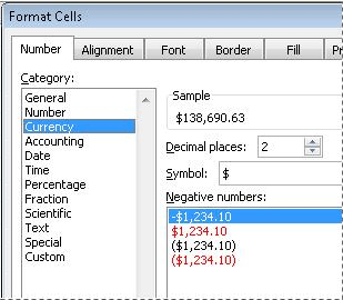
The Number tab allows you to format the way that your numbers will be displayed. You can choose from options such as percentages, dates, currency, times, etc.

Start by selecting the cells you want to modify.
On the Home tab, select Format > Format Cells, which will open the Format Cells dialog box.
The first tab listed is the Number tab. The Category list in the Number tab allows you to select the format you want to use, such as Date, Time, Percentage, Currency, etc. You will also have the option to further customize your selection. For example, you could select a specific way that you’d like to represent negative currency values (see image below).

Source: Microsoft Support

Alignment Tab

Automatically, Excel formats any text to the bottom-left of a cell and numbers to the to the bottom-right. The Alignment tab within the Format Cells dialog box allows you to customize the way that you’d like your values to be aligned, both Vertically or Horizontally.

Should you require a more dramatic text alignment, the Degrees field allows text to be oriented 90 degrees in either direction up or down.

Text Control allows you to control the way Excel formats information in a cell. There are three types of text control: wrapped text, shrink to fit, and merge cells.

Should you require a more dramatic text alignment, the Degrees field allows text to be oriented 90 degrees in either direction up or down.

Text Control allows you to control the way Excel formats information in a cell. There are three types of text control: wrapped text, shrink to fit, and merge cells.

And finally, Text Direction switches the direction of the worksheet—in other words, column A could start from the upper right side instead of the upper left.

To make any of these modifications, first select the text that you’d like to modify.
On the Home tab, select Format > Format Cells, which will open the Format Cells dialog box.
Click on the Alignment tab. From there, you will see Text Alignment (Horizontal; Vertical), Text Control (Wrap text, Shrink to fit, Merge cells) and Text Direction (Context; Left-to-Right; Right-to-Left).

Font

Quick Font changes can be made directly from the Home tab, but for mass changes, it’s more efficient to use the Format Cells dialog box. From there, it’s easy to change typeface, point size, font size, bold, italicize, underlining, and color across an entire selection of cells.

To make any of these modifications, first select the text that you’d like to modify.
On the Home tab, select Format > Format Cells, which will open the Format Cells dialog box.
Clicking on the Font tab will prompt the possible selections, as well as a preview of your changes.

Border

Excel allows you to construct borders around a single cell or a range of cells. You can determine where the lines will be drawn (for example, only the top of the cell or on all horizontal sides) and adjust their thickness, color, and line style.

To make any of these modifications, first select the text that you’d like to modify.
On the Home tab, select Format > Format Cells, which will open the Format Cells dialog box.
Clicking on the Border tab will prompt the possible selections. If you want to remove a specific border, click the button for that border a second time.If you want to change the line color or style, click the style or color that you want, and then click the button for the border again.

Fill

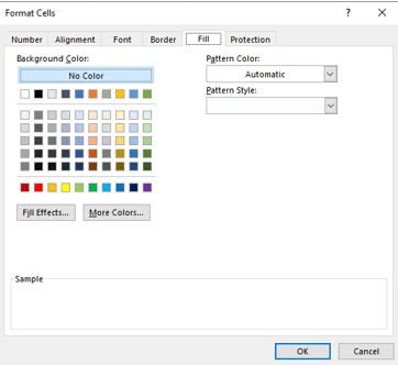
The Fill tab in the Format Cells dialog box allows users to set the background color of all selected cells, which may include applying two-color patterns or shading from the Patterns option. Here’s how to shade cells with Patterns:

Start by selecting the text that you’d like to modify.
On the Home tab, select Format > Format Cells, which will open the Format Cells dialog box.
Click on the Fill tab, then select the Pattern Style you’d like to set as the background to your cells. As an optional addition, you may also choose to set a Pattern Color to accompany your Pattern Style.
At any time, you can return to the default state of your selected cells by choosing No Color at the top of color selection.

Protection

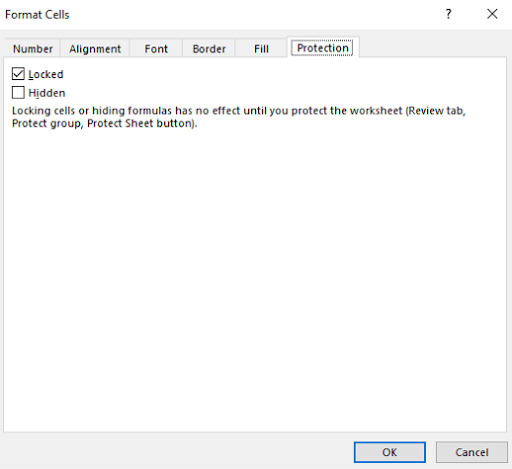
The Protection tab does not apply unless you have already protected your worksheet. To do so, click on Protection in the Tools menu, select Protect Sheet, and then select the Contents check box(es) to determine how, exactly, the worksheet will be protected.

When the Locked option is selected, you are prohibited from doing the following:

Changing the cell data or formulas.
Typing data in an empty cell.
Moving the cell.
Resizing the cell.
Deleting the cell or its contents.

When the Hidden option is selected, that means that all formulas used to calculate values will no longer be viewable in the formula bar (however, you can still see the end result of that formula).

Recycling Excel File Formats

After you’ve formatted your Excel worksheet exactly how you want it using the six primary Excel file formats, odds are, you don’t want to keep repeating that work. Here are some of the ways that users can recycle their Excel formatting process.

Copying Styles Between Workbooks

With each new worksheet, there’s a way to copy over previous Excel file formats from an original worksheet.

First, open the workbook with your original Excel formatting and the new workbook.
From the original workbook, click Cell Styles in the Styles group on the Home tab.
Choose Merge Styles at the bottom of the gallery.
In the resulting dialog, select the open workbook that contains the styles you want to copy.
Click OK twice.

Copy Over Formats

Sometimes you just want to copy over formatting from one column to another (without the values). In that scenario, it’s easy to copy over formatting only.

First, start by selecting the destination cell or range of cells.
Then, right-click the border of the cell with your preferred formatting and drag it to the target cell or range of cells.
When you release the mouse, Excel will display a submenu where you can select “Copy Here,” “Copy Here as Values Only” or “Copy Here as Formats Only.” In this case, you’d want to select the third option, leaving the cells blank but prepped with the correct formatting.

Use Paste to Copy Formatting

In a similar vein, you can use the Paste function to copy over formatting from one column to another.

You’ll start by selecting and copying [Ctrl]+C your original cell or range of cells.
Then, click anywhere instead your destination cell or range of cells. Press [Ctrl]+[Spacebar] to select the entire column or [Shift]+[Spacebar] to select the entire row.
Once you’re ready to paste over the formatting, choose Formatting from the Paste drop-down.
Live Preview will show you what the applied formats will look like, and you can click OK if everything looks good.

Follow Me

If you like my post please follow me to read my latest post on programming and technology.

Instagram

Facebook

Abdul Quadir